Analyzer Sample Lag Time Calculation Basics: What You Need to Know to Reduce Uncertainty

To consistently obtain representative samples for an analyzer, your grab sampling system needs to be designed with an accurate understanding of the process conditions, flow, volume, and the time (lag) required to flush out any stagnant fluids that remain in sample transport lines. If you’re not familiar with how sampling system components such as tubing, valves, elbows, and tees influence lag time calculations, it’s best to engage the help of an experienced fluid systems engineer. With that guidance, you can be assured the critical lag time calculation will be correct and you’ll consistently be capturing representative samples to send to the analyzer. 

To give you an appreciation of the various factors to be considered in the calculation, let’s explore how key components affect the calculation. In the explanation below I’m focusing solely on liquid samples. Gas sample calculations require additional factors when calculating analyzer lag times.

Sample Tap Location and Design

The sample tap/probe should be located at a point of higher pressure than the return point to ensure proper flow. The sample probe should be installed in a vertical pipe run and extend into the pipe ⅓ of the inside diameter. If the differential pressure drop is insufficient, a centrifugal pump needs to included in the design, and its volume and flow will be part of the analyzer sample lag time calculation. 

Minimize or Eliminate Dead Volume 

Dead volumes or spaces (sections in the sampling system where fluids are trapped and don’t flow smoothly) can consistently contaminate sample quality. Between samplings, fluids will stagnate in tee fittings. Sharp edges on fittings disrupt the smooth flow. A well-designed sampling system will eliminate or at least minimize dead space sections and minor losses due to sharp edges. If dead space sections are unavoidable, a system purge or extended flow time or sweep before taking the sample needs to be factored into the lag time calculation. 

Dead volumes can often be eliminated by designing the sampling system to have a continuous flow in all lines and using a three-way valve to direct sample fluid flow before, during, and after the sample is taken. The volume and flow of each valve used in the design will be part of the lag time calculation.

Sample Transport Line

Distance between the sample port and the sample station tap, tubing diameter, and any components along the way are all critical parameters in analyzer sample lag time calculations. In ideal circumstances, the distance between tap and sampling station is minimized. However, in many retrofit grab sampling installations that must accommodate existing infrastructure, that distance may be significant. 

Other transport components that influence lag time include filters that affect flow and coolers or heat exchangers required to deliver samples, such as high-temperature hydrocarbons, at safe temperatures.  

Analyzer Sample Lag Time Calculation

At its simplest, the analyzer sample lag time calculation is the sum of total volumes (using internal diameters) of the transport tubing and components divided by their flow rates. Let’s walk through two relatively simple examples of the calculation.

lag time = component volume / sample flow rate

For tubing: time = volume x length / flow 

Example: A 50’ length of 0.25” tubing (5 cm³ per foot) has a volume of 250 cm³. With a flow rate of 500 cm³ per minute, the lag time is 30 seconds prior to capturing a representative sample.

For components: volume = device 𝛑r² x length / flow 

Example: a filter with diameter of 2” and length of 2” has a volume of 3.14 x 1² x 2 x 16.28 (cm³/cu inch) = 51.15 cm³. With a flow rate of 500 cm³ per minute, the lag time is approximately 6 seconds.

When calculating the lag time for components, a best practice recommends multiplying the volume by a factor to allow for enough time to thoroughly displace any stagnant fluid in the component with fresh process fluid. The recommended factor is 3x the volume to ensure you are capturing a truly representative sample. Applying that factor to the component formula results in a lag time of 18 seconds.  

In the simplified examples given above, the total lag time for tubing and filter would be at least 73 seconds.

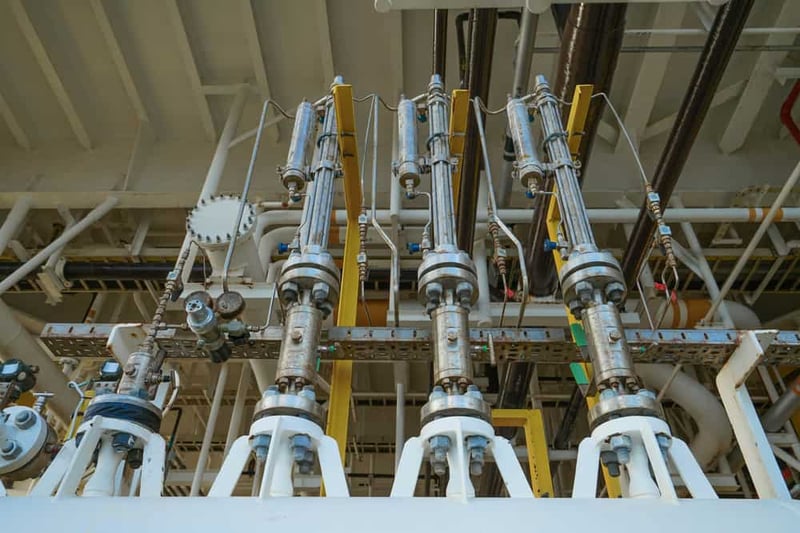
Most grab sampling systems are a bit more complicated as depicted in the image. Volume and flow calculations need to be made for each component in the sample transport line. Beyond the physical properties of the transport components, you’ll also need to factor differences in liquid vs. gas samples, varying process pressures and ambient temperatures, fluid compressibility, purging, and closed vs. fast loop designs in the calculation. 

Why It’s Critical To Accurately Calculate Analyzer Sample Lag Time 

A grab sampling system is a liability when the analyzer sample lag time is inaccurate. Too much time and you’re wasting process fluid and time. Multiply that error by the number of samples taken annually and the number of sample stations, factoring in inaccurate calculations; the costs can be considerable. Too little time and you fail to properly clear the sample transport line of stagnant fluid and risk contamination of every sample. That’s why it’s critical to get analyzer sample lag time calculations correct. 

Swagelok is a trusted resource for designing, assembling, and testing grab sampling systems. We draw our expertise from engineers worldwide who regularly consult with chemical and petroleum, oil and gas, utility, and semiconductor industries. We believe that the best grab sampling system designs begin with an onsite consultation to assess the process conditions, infrastructure, and type of analysis. Using that information, we’ll then design the grab sampling system for those requirements and, of course, the analyzer sample lag time calculation will be an essential part of the design. 

Whether it’s a simple non-toxic liquid sampling into a bottle for transport to an on-site analyzer or a more complicated high-pressure, high-temperature hydrocarbon sample involving system purging, process fluid cooling, and capture using a pressurized cylinder at a sampling station 150 feet from the sample tap, our field engineers bring a wealth of industry and process knowledge to design reliable grab sampling systems that consistently deliver representative samples.

To find out more about how Swagelok Northern California can work with you to design, grab sampling systems that accurately calculate sample lag times to help ensure representative samples, contact our team today by calling 510-933-6200.

Morgan Zealear | Product Engineer – Assembly Services

Morgan holds a B.S. in Mechanical Engineering from the University of California at Santa Barbara. He is certified in Section IX, Grab Sample Panel Configuration, and Mechanical Efficiency Program Specification (API 682). He is also well-versed in B31.3 Process Piping Code. Before joining Swagelok Northern California, he was a Manufacturing Engineer at Sierra Instruments, primarily focused on capillary thermal meters for the semiconductor industry (ASML).